Posts

Apr 6, 2016 NEW!

CI Project1: [Neural Networks] Multi-Layer Perceptron Based Classifier

In this Computational Intelligence and Applications project, we were asked to implement multi-layer perceptrons and experiment with them as classifiers. Test data are two-dimentional points and classified into class 1 or 2.

Environment

Python 3.5 with library matplotlib 1.5.1(for ploting figures)
Running on OSX 10.11 with Intel Core i5 2.6GHz & 8GB 1600Mhz DDR3 or AWS Ubuntu Server 14.04 64bit (instance type: t2.micro)

Methodology

Use online version of backpropagation algorithm since it’s been told^[2] to be better than batch version.
In total of 400 data points from two files, take 320~360 as training set and the remaining as validation set.
The activation function is the logistic function.
The neural network consists of 2 layers, 1 hidden layer + 1 output layer.
The number of neurons of hidden layer is 4. (will be explained later)
Learning rate η is initially set to 0.05, and adjusted to 0.01 later on.
The stopping criterion is running 10,000 epochs or 100,000 epochs, depending on the number of hidden neurons (to avoid long running time).
Momentum term is integrated later.

Experiments

First, try several different numbers (i.e., 32, 16, 8, 4, 2) of neurons in the hidden layer to choose the best model, which is having 4 hidden neurons in the hidden layer.

(PS. HN: hidden neuron, LR: learning rate, TS: Training set, VS: validation set, MA: alpha term in momentum)

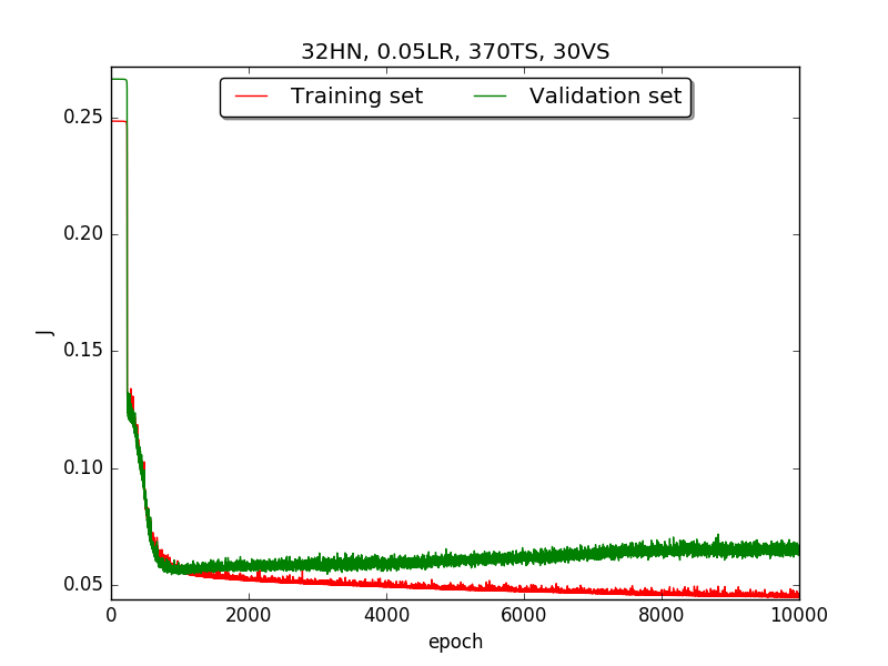
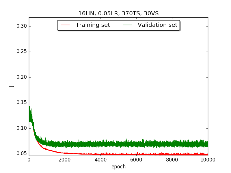
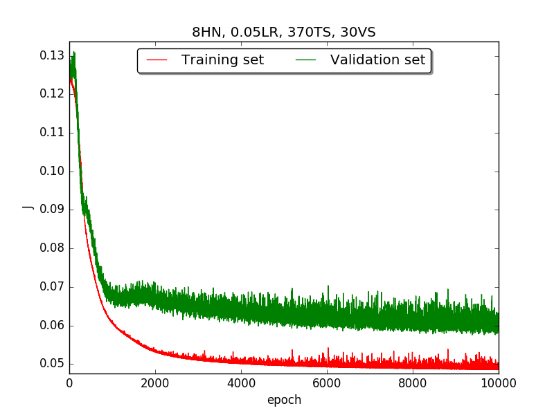
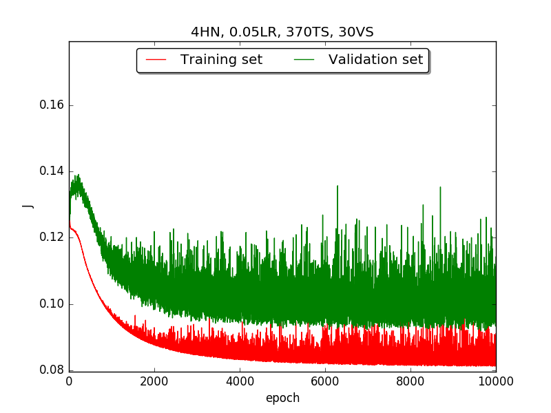
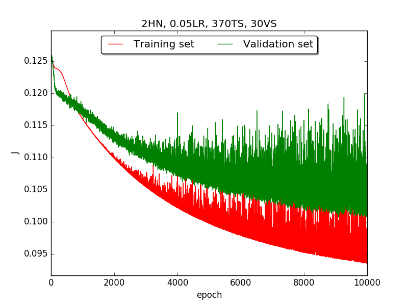
←↑ Results of running 10,000 epochs on a NN of HN(32, 16, 8, 4, 2) neurons in the hidden layer, 0.05 learning rate, 370 data points in training set, 30 data points in validation set and no momentum term

Second, since the amplitude of oscillation in the above figures is too large, I deceided to run the experiment again with lower learning rate, that is, 0.01 to see if it will get better.

Also, adjust the ratio of the size of training set to the size of validation set to 80:20 (i.e., 320TS & 80VS), which is the recommended ratio.

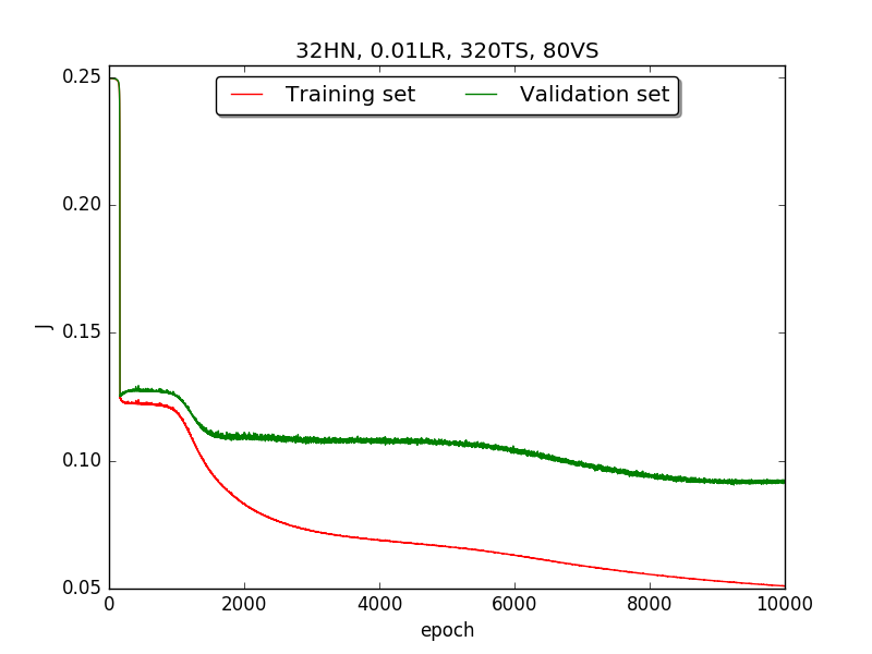
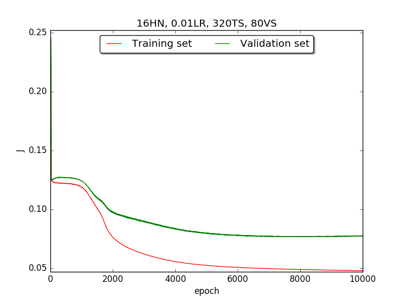
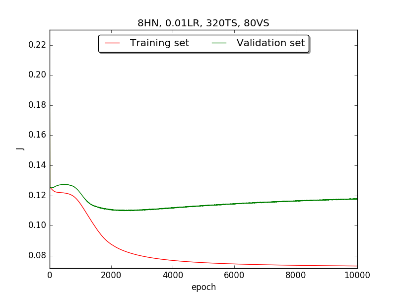
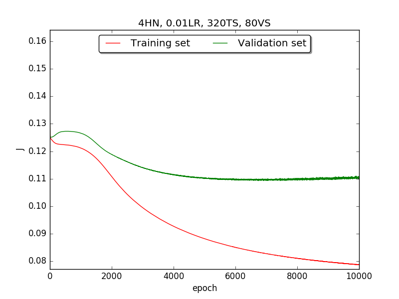
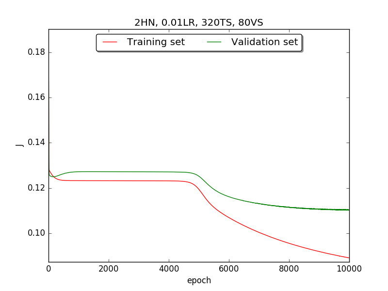
←↑ Results of running 10,000 epochs on a NN of HN(32, 16, 8, 4, 2) neurons in the hidden layer, 0.01 learning rate, 320 data points in training set, 80 data points in validation set and no momentum term

Third, integrate momemtum into the neural network and highlight the first epoch that satisfy the early stopping criterion (shown as blue veritcal line with epoch number).

Moreover, since the number of neurons has chosen to be 4, increase the stopping criterion to 100,000 epochs to get more precise result.

Also, I noticed that learning curves in second step is quite strange and I suspected that it’s because the training set is too small to achieve the correct model. Therefore, I tweaked the TS:VS ratio to 90:10 (i.e., 360TS & 40VS).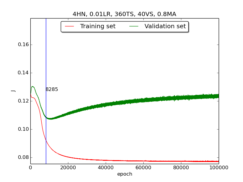

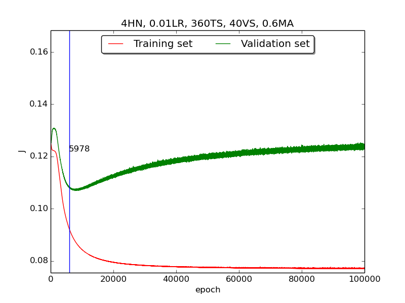
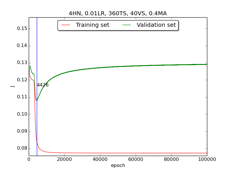
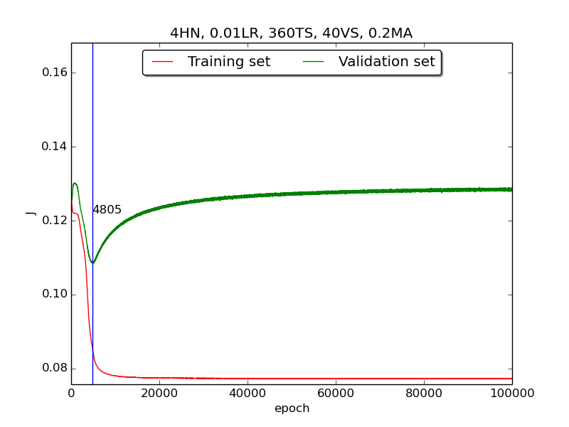
↑ Results of running 100,000 epochs on a NN of 4 neurons in the hidden layer, 0.01 learning rate, 360 data points in training set, 40 data points in validation set, MA(0.8, 0.6, 0.4, 0.2) momentum term and early stopping highlight

Analysis

[1] In the first part, I think the reason of causing the large amplitude of oscillation is that I set the learning rate too high(0.05). Therefore, when in the second part with lower learning rate(0.01), the amplitude of oscillation reduced significantly.

[2] As one can see in first & second part, when the number of hidden neuron is equal or larger than 4, the shape of the learning curve becomes similar. Therefore, according to Ockham's Razor^[3], I selected the simplest one - 4 neurons in the hidden layer.

[3] For the third part, I integrated the momentum term and the expected learning curve (i.e., after certain amount of time, the error of validation set increases due to overfitting the training set) has finaly shown.
To investigate more deeply, I supposed that if first & second had more time (i.e., run with more epochs), they would have the same result as third and did another experiment that runs 100,000 epochs with no momentum. It turned out that the supposition is correct! The reason the learning curve was not obvious was that the running time wasn’t enough.
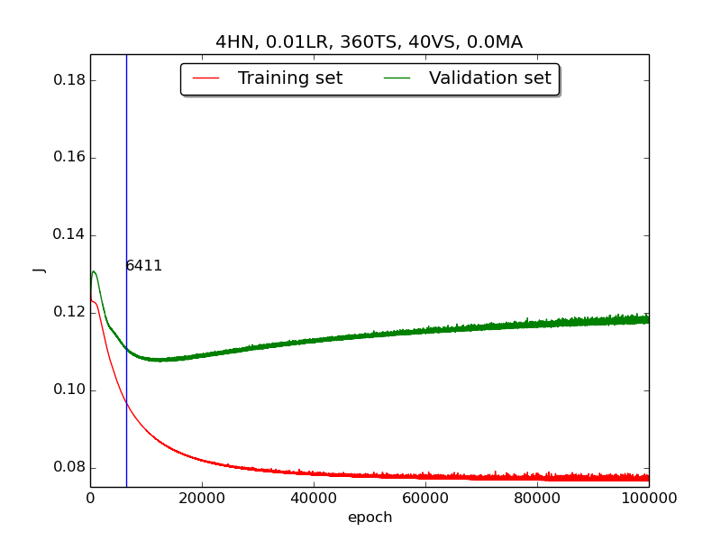↑ Results of running 100,000 epochs on a NN of 4 neurons in the hidden layer, 0.01 learning rate, 360 data points in training set, 40 data points in validation set and no momentum term

[4] For the third part, the four figures testified that the higher momentum is, the larger the amplitude of oscillation becomes.

[5] However, in the third part, some unexpected results had shown. As far as I know, the higher momentum should have led to the increase of speed of convergence. Nevertheless, according to the figures in thrid, the least epoch satisfying early stopping criterion is when momentum = 0.4 instead of 0.8. I think the reason was the different (resulting from randomness) choice of initial biases.

[6] As for normalization, I transformed all the points classified as 2 to 0 due to the output of activtion function (between 0~1, inclusive).

Ref / Note

[1] Code ref: A Step by Step Backpropagation Example – Matt Mazur

[2] Understanding Neural Network Batch Training: A Tutorial – Visual Studio Magazine

[3] Occam’s razor on Wikipedia

Source → cyhuang1230/NCTU_CI

Please look for HW1.py.

Mar 24, 2016
BDATAA Project1: Analyzing NYC Taxi Data

In this Big Data Analytics Techniques and Applications project, we were asked to analyze 3-month NYC taxi data (about 5.5GB, 35,088,737 data points). I will only mention the most crucial and difficult problem, which is:

What are the top pickup/dropoff regions?

[ANSWER]
Pickup region:
Centroid at 40°45’20.1”N 73°58’56.6”W (longitutde = -73.98239742908652, latitude = 40.75556979631838) with radius r = 21.86850019225871, total 14,815,015 pickups included.

Dropoff region:
Centroid at 40°45’07.2”N 73°59’04.1”W (longitutde = -73.98447812146631, latitude = 40.75200522654204) with radius r = 27.07032741216307, total 17,186,117 dropoffs included.

** Note: r is calculated based on the formula sqrt(longitude_diff^2+latitude_diff^2), which I believe is meaningleass and should be converted to km. (I will do that sometime :P)

[DISCUSSION]
I implemented k-means clustering^[1] to solve this problem. However, there’s a serious pitfall regarding this algorithm: how to choose k?
To resolve this, I tried to list all possible k’s, ranging from 1~10 (for all three-month data) or 1~50 (for limited amount of data), and chose the k when SSE-k function becomes “flat”.
(k 的選擇: 選擇當 SSE-k 函數趨近平緩時的k點)
→ Finally, choose k = 5 to do the clustering.

Result for different k’s (-1 data points means not limited):

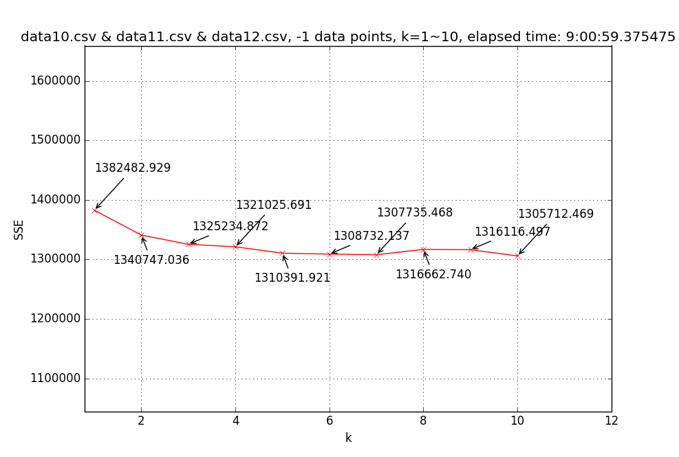↑ Line chart of SSE(sum of square error) with different k’s (1~10) based on three-month (Oct.~Dec.) pickup region data (35,088,737 data points).

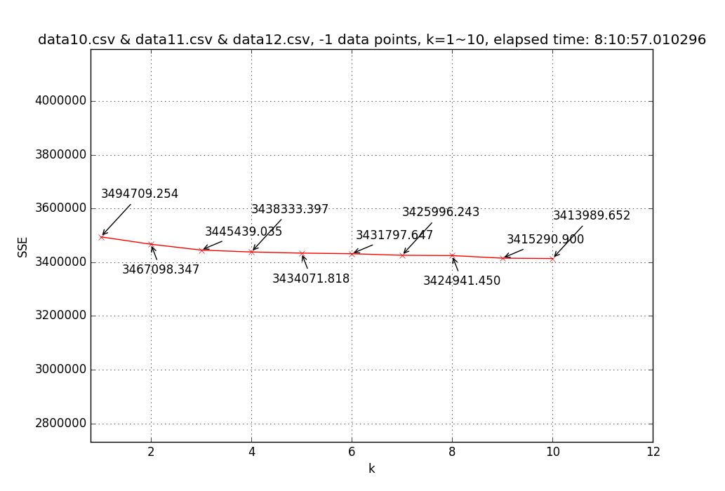↑ Line chart of SSE with different k’s (1~10) based on three-month (Oct.~Dec.) dropoff region data (35,088,737 data points).

Result for pickup data with k = 5:
```
==> 5 clusters with SSE = 1310382.527, total 10 iterations, duration: 0:58:44.093826
-------------
[k = 5] Centroid #0 @(-73.98239742908652,40.75556979631838) with r = 21.86850019225871 [14815015 points]
[k = 5] Centroid #1 @(-73.78023972555476,40.64441273159325) with r = 260.35266030662689 [805122 points]
[k = 5] Centroid #2 @(-73.96136756589190,40.78012632758659) with r = 23.04849337580119 [8147234 points]
[k = 5] Centroid #3 @(-73.99744188868137,40.72594059025759) with r = 662.30254596214866 [9716760 points]
[k = 5] Centroid #4 @(-73.87396560811541,40.76951321876881) with r = 33.88323463224077 [1095900 points]
```
→ Choose Centroid #0 @(-73.98239742908652,40.75556979631838) with r = 21.86850019225871 [14815015 points]

Result for dropoff data with k = 5:
```
==> 5 clusters with SSE = 3431839.916, total 36 iterations, duration: 3:28:30.800414
-------------
[k = 5] Centroid #0 @(-73.76951586370677,40.65764030599616) with r = 260.34678752815660 [463269 points]
[k = 5] Centroid #1 @(-73.98447812146631,40.75200522654204) with r = 27.07032741216307 [17186117 points]
[k = 5] Centroid #2 @(-73.95882476626755,40.78457504343687) with r = 439.94876239844325 [8876526 points]
[k = 5] Centroid #3 @(-73.99645795122916,40.71086509646405) with r = 695.53686724899160 [6822543 points]
[k = 5] Centroid #4 @(-73.88058752281310,40.76332250437670) with r = 35.03531452510111 [1260853 points]
```
→ Choose Centroid #1 @(-73.98447812146631,40.75200522654204) with r = 27.07032741216307 [17186117 points]

Source → cyhuang1230/NCTU_BDATAA

Please look for HW1_q1.py.
To try:
[1] Download taxi data^[2] and rename to data10.csv, data11.csv, data12.csv separately.
[2] Run python3.5 HW1_q1.py

Note / Ref.

[1] k-means clustering: A Programmer’s Guide to Data Mining

[2] Taxi data can be downloaded here: October, November, December
Jan 8, 2016
NP HW4: SOCKS4 Server & Client

In this network programming homework, we are asked to build SOCKS4 server and client and combine HW3 to demo.

Spec is not included; however, the basic architecture can be illustrated as follows:

There are some notable ideas I came up with:

For SOCKS client (CGI):
- Same as HW3. Just need to send SOCK4 requset and handle SOCK4 reply.
For SOCKS Server:

- CONNECT mode procedure:
```
accept → read SOCKS req → check firewall rules →
connect to dest host → send SOCKS reply → redirect data
```
- BIND mode procedure:
```
accept → read SOCKS req → check firewall rules →
bind socket → listen → send SOCKS reply → 
accpet from server → send SOCKS reply (to original client) → redirect data
```
- When redirecting data, should avoid using strncpy since it may contain '\0' in data, which occasionally leads to data error (less bytes are copied than expected).
- When bind with system-assigned port, give 0 to sockaddr_in.sin_port.

Demo video:

Source → cyhuang1230/NetworkProgramming

For SOCKS client (CGI):
Please look for NP_project4_Server.cpp.
To try: make hw4_cgi , upload to a HTTP server and run <BASE_URL>/hw4.cgi.

For SOCKS server:
Please look for NP_project4_Server.cpp.
To try: make hw4_server and run ./np_hw4.
Dec 24, 2015
NP HW3: Remote Batch System (RBS)

In this network programming homework, we are asked to build a Remote Batch System (RBS). It’s actually a combination of client and server, whose diagram can be drawn as follows:

As required in spec(hw3Spec.txt), we have to write three programs:
1. CGI: a webpage(hw3.cgi) that displays server’s response dynamically.
2. HTTP Server: a cpp program that runs as a HTTP server.
3. Winsock: a combination of 1. and 2. but using Winsock.
For more details, please refer to hw3Spec.txt in the repository (cyhuang1230/NetworkProgramming).

There are some notable ideas I came up with and described as follows.

For CGI (Part I):
- Write may fail. Write a wrapper class to handle this.
- Parsing query string needs to be handled carefully.
- Since we’re client now, doesn’t matter which port to use, i.e. no need to bind anymore!
- Try using flag(bitwise comparison) instead of individually specifying each property in log function.
- Output recerived from servers should be handled(e.g. \n, <, >, &, ', ") since JavaScript has different escape characters than C. Also, the order of processing characters matters.
- Most importantly, non-blocking client design.
      [1] connect may be blocked due to slow connection.
          => Set O_NONBLOCK to sockfd
      [2] Client program may block (e.g. sleep)
          => Don’t wait for response (i.e. read) after write to server. Instead, use select to check when the response is ready to read.
For HTTP Server (Part II):
- Use select to accept connections.
- Fork a child process to handle request.
- Plain text file can be read & write directly. Content type needs to be set properly.
- CGI needs to be execed. => dup its STDOUT_FILENO to sockfd.
For Winsock (Part III):
- Same logic as Berkeley Socket version.
- To read file, use ReadFile instead of ReadFileEx (I encountered pointer error)
- Keep track of doneMachines. When done (== numberOfMachines), close socket and print footer.
- I like Berkeley Socket much more than Winsock :(
Demo video:

Source → cyhuang1230/NetworkProgramming

For part I (CGI):
Please look for NP_project3_1.cpp.
To try: make hw3_1_debug, upload to a HTTP server and run <BASE_URL>/hw3.cgi.

For part II (HTTP Server):
Please look for NP_project3_2.cpp.
To try: make hw3_2_debug and run ./np_hw3.

For part III (Winsock):
Please look for NP_project3_3.cpp. Run with Visual Studio is recommended.
Nov 23, 2015
NP HW2: Remote Working Ground (RWG)

In this network programming homework, we are asked to build a remote working ground (RWG), which is actually a combination of hw1 and chat & public pipe function.

According to the spec(hw2Spec.txt), we need to write two programs:
1. Use the single-process concurrent paradigm.
2. Use the concurrent connection-oriented paradigm with shared memory.
For more details, please refer to hw2Spec.txt in the repository (cyhuang1230/NetworkProgramming).

There are some notable ideas I came up with and described as follows.
(I will start with version II since I wrote that first :P)

For concurrent version:
- Keep track of client’s data (e.g. sockfd, pid…) so that we can send msg to each client.
- Store client data & messages in shared memory so let every child can read.
- Create additional MAX_USER(# of user) blocks of shm to store direct msg (or broadcst msg).
- There’s no way server can be closed properly (must end by Ctrl+C), so, in order not to leave any shm unrelaesed, we won’t shmget until the first client is connected, and free shm when all clients are disconnected.
  → To keep track of the number of children, sa_handler needs to be implemented separately.
  → Furthermore, MUST reset sa_handler in the child process so that won’t mistakenly detach shm later when exec.
- Use signal SIGUSR1 to notify other process there’s a new msg to write.
- Semaphore on public pipes to prevent concurrent issue. (Same create/release idea as shm.)
- Use FIFO, a.k.a Named pipe, to implement public pipe. [No need to store in shm].
- Implement a generic function to send msg to a specific user.
  Function hierarchy:
  → sendRawMsgToClient → tell
  → sendRawMsgToClient → broadcastRawMsg → yell/name/who
For single-process version:
- Basically same structure as ver. II, but as a single-process program, we don’t need any shm or semaphore, which makes it much easier, yayyy!.
- Only involves one huge adjustment.
  Consider the following input:
```
[Client 1] % ls |1
[Client 2] % ls |1
[Client 1] % cat
[Client 2] (empty) <- stucked, prompt won't display
```
    This error is caused by the way we decide input.
    → We can no longer expect the whole input with numbered-pipe can be got in one while loop.
    → Instead, we have to check input line by line, and keep track of input-related information.

Demo video: (client is not included in the repo)

Source → cyhuang1230/NetworkProgramming

For ver. I (Single process):
Please look for NP_project2_Single.cpp.
To try: make hw2s and run ./np_hw2s.
*Try with debug message: make hw2_debugs and run ./np_hw2s.

For ver. II (Concurrent):
Please look for NP_project2_Concurrent.cpp.
To try: make hw2 and run ./np_hw2.
*Try with debug message: make hw2_debug and run ./np_hw2.

*Debug version is complied with -g, which may use gdb np_hw2(s) to debug.
Nov 2, 2015
NP HW1: Remote Access System (RAS)

In this network programming homework, we were asked to build a remote access system. It’s kind of like a shell on the server side.

For more details, please refer to hw1Spec.txt in the repository (cyhuang1230/NetworkProgramming).

Demo video:

Source → cyhuang1230/NetworkProgramming

Please look for NP_project1.cpp.
To try: make hw1 and run ./np_hw1.
Try with debug message: make hw1_debug and run ./np_hw1.
Aug 12, 2015
CYHPOPImageButton Released!

CYHPOPImageButton is a library written in Swift 2.0, offering you a cute, bouncy image iOS button (Facebook Messenger stickers-alike), implemented with Facebook pop.

Demo video:

Source → cyhuang1230/CYHPOPImageButton