NCTU Computational Intelligence and Application Projects
Projects I’ve worked on in graduate-level course Computational Intelligence and Application(計算型智慧與應用) in NCTU in Spring 2016.
This course will be completed in June, 2016. Total 4 projects expected.
-
CI Project1: [Neural Networks] Multi-Layer Perceptron Based Classifier
In this Computational Intelligence and Applications project, we were asked to implement multi-layer perceptrons and experiment with them as classifiers. Test data are two-dimentional points and classified into class
1or2.Environment
Python 3.5with librarymatplotlib 1.5.1(for ploting figures)- Running on
OSX 10.11 with Intel Core i5 2.6GHz & 8GB 1600Mhz DDR3orAWS Ubuntu Server 14.04 64bit (instance type: t2.micro)
Methodology
- Use online version of backpropagation algorithm since it’s been told[2] to be better than batch version.
- In total of 400 data points from two files, take 320~360 as training set and the remaining as validation set.
- The activation function is the logistic function.
- The neural network consists of 2 layers, 1 hidden layer + 1 output layer.
The number of neurons of hidden layer is 4. (will be explained later) - Learning rate η is initially set to 0.05, and adjusted to 0.01 later on.
- The stopping criterion is running 10,000 epochs or 100,000 epochs, depending on the number of hidden neurons (to avoid long running time).
- Momentum term is integrated later.
Experiments
First, try several different numbers (i.e., 32, 16, 8, 4, 2) of neurons in the hidden layer to choose the best model, which is having 4 hidden neurons in the hidden layer.
(PS. HN: hidden neuron, LR: learning rate, TS: Training set, VS: validation set, MA: alpha term in momentum)
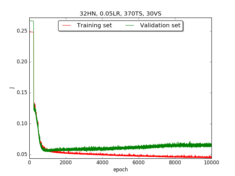
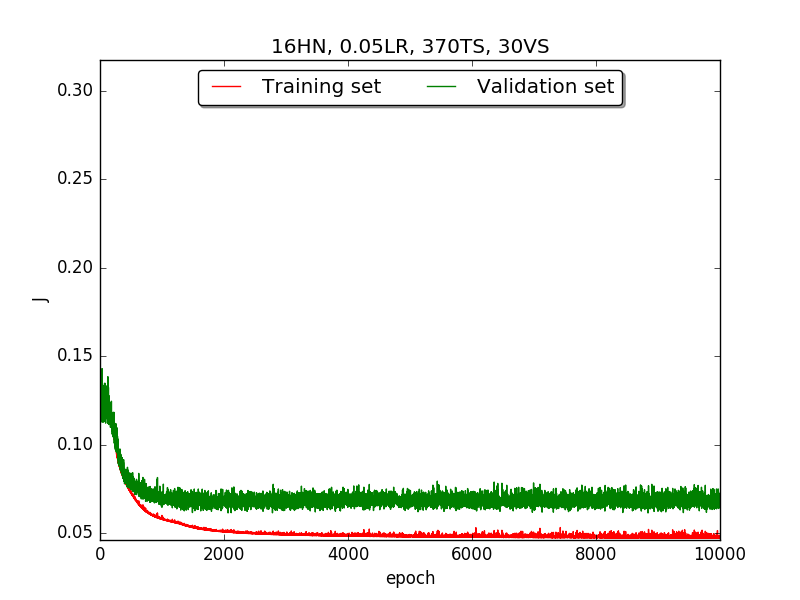
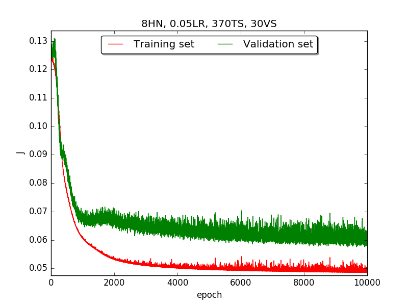
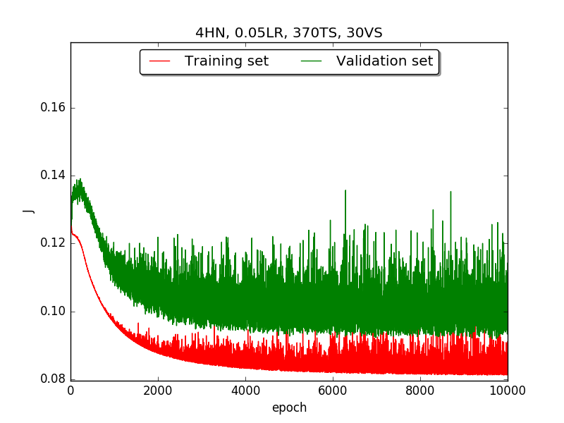
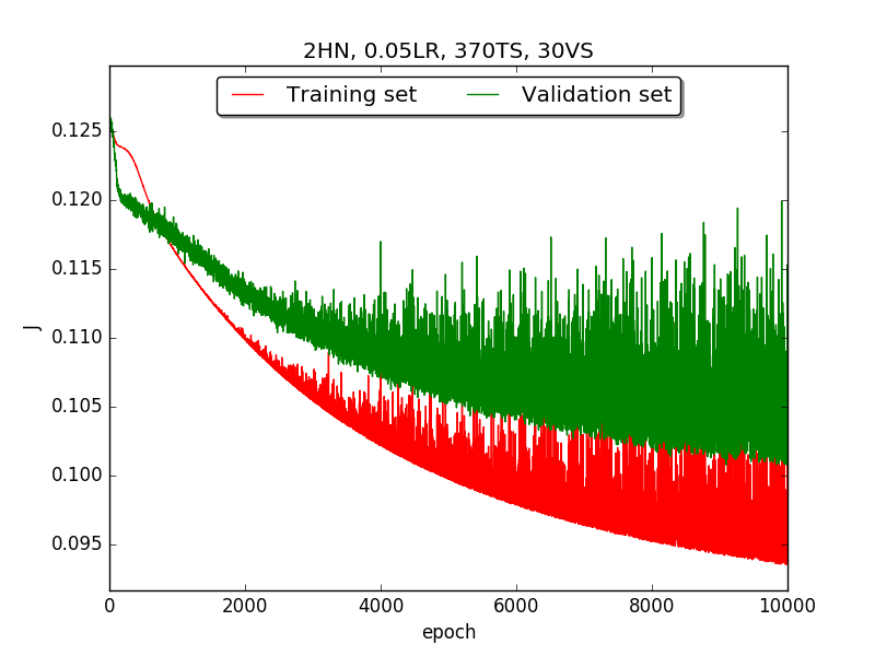
←↑ Results of running 10,000 epochs on a NN of HN(32, 16, 8, 4, 2) neurons in the hidden layer, 0.05 learning rate, 370 data points in training set, 30 data points in validation set and no momentum term
Second, since the amplitude of oscillation in the above figures is too large, I deceided to run the experiment again with lower learning rate, that is, 0.01 to see if it will get better.
Also, adjust the ratio of the size of training set to the size of validation set to 80:20 (i.e., 320TS & 80VS), which is the recommended ratio.
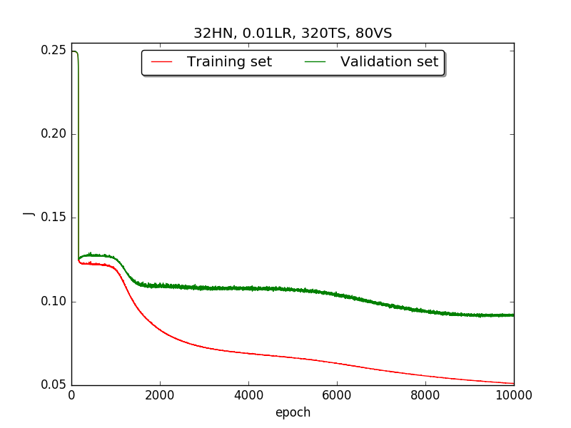
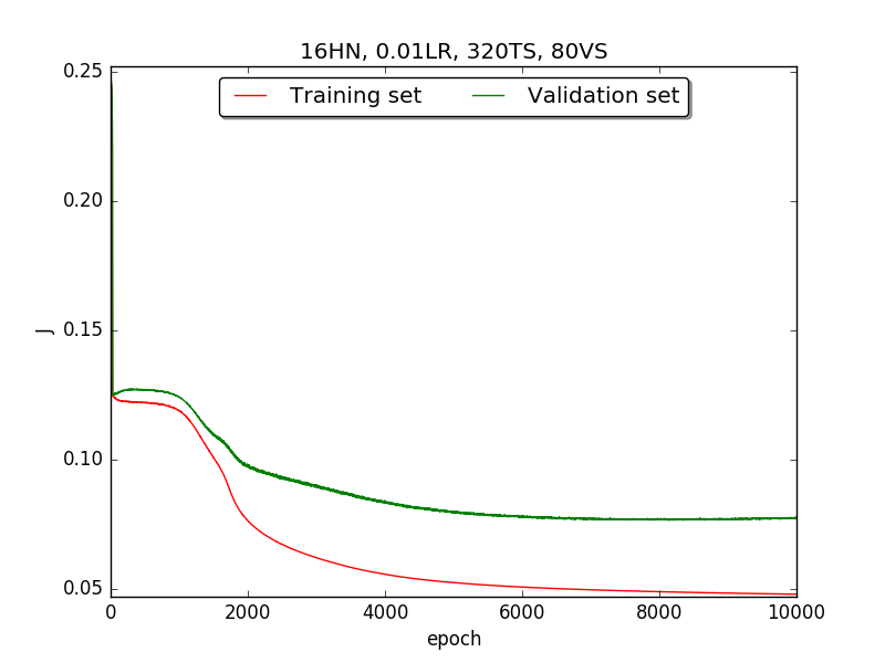
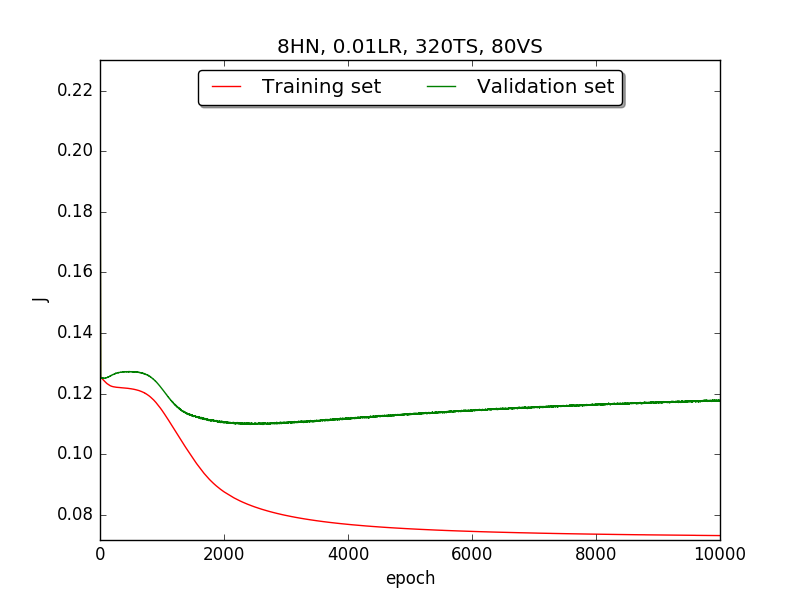
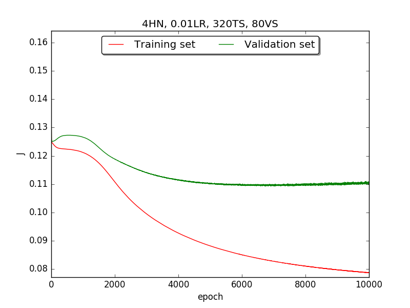
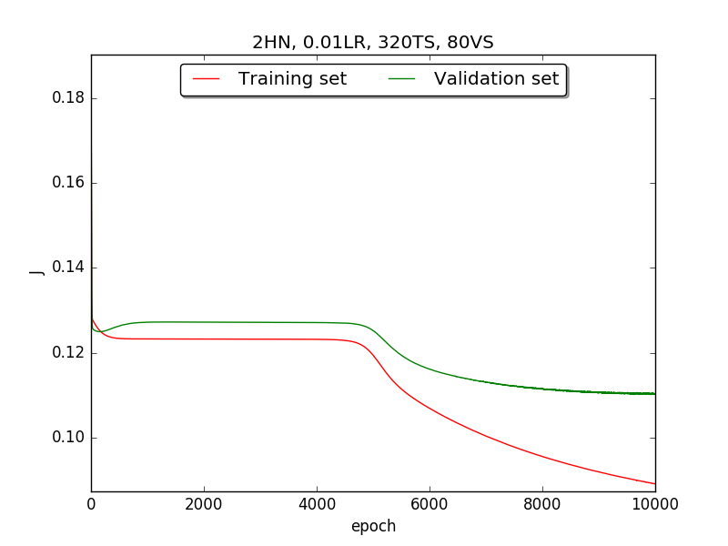
←↑ Results of running 10,000 epochs on a NN of HN(32, 16, 8, 4, 2) neurons in the hidden layer, 0.01 learning rate, 320 data points in training set, 80 data points in validation set and no momentum term
Third, integrate momemtum into the neural network and highlight the first epoch that satisfy the early stopping criterion (shown as blue veritcal line with epoch number).
Moreover, since the number of neurons has chosen to be 4, increase the stopping criterion to 100,000 epochs to get more precise result.
Also, I noticed that learning curves in
secondstep is quite strange and I suspected that it’s because the training set is too small to achieve the correct model. Therefore, I tweaked the TS:VS ratio to 90:10 (i.e., 360TS & 40VS).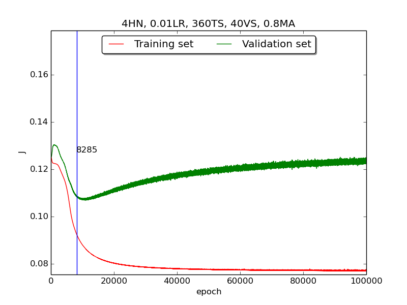
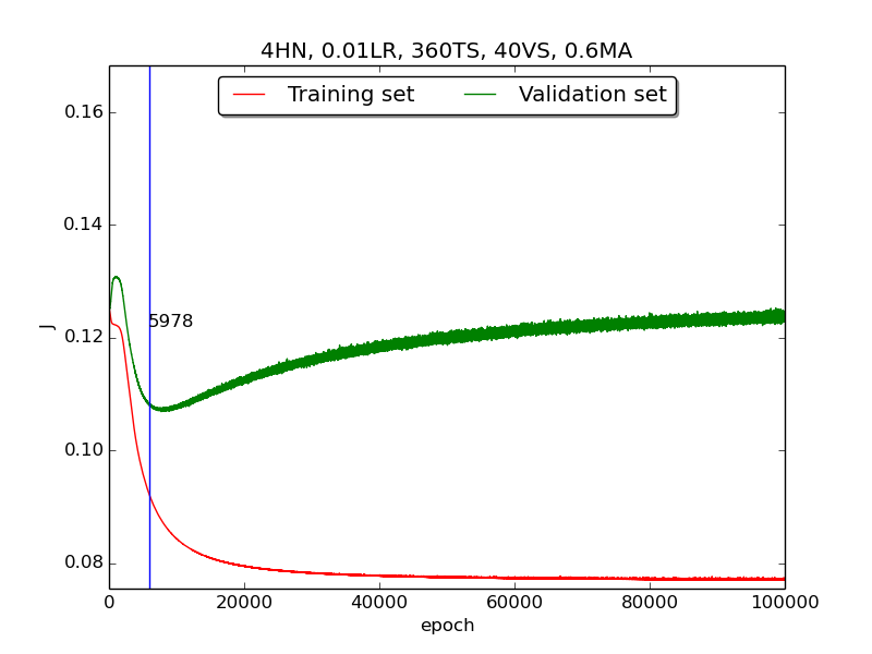
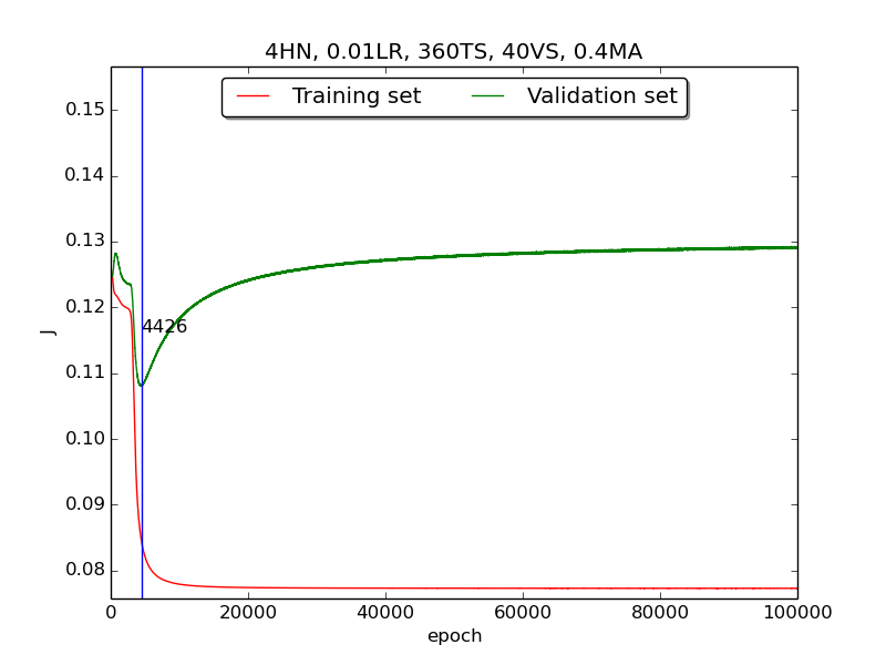
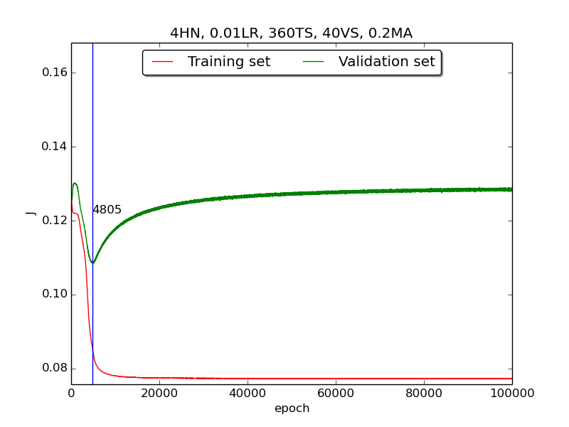
↑ Results of running 100,000 epochs on a NN of 4 neurons in the hidden layer, 0.01 learning rate, 360 data points in training set, 40 data points in validation set, MA(0.8, 0.6, 0.4, 0.2) momentum term and early stopping highlight
Analysis
[1] In the
firstpart, I think the reason of causing the large amplitude of oscillation is that I set the learning rate too high(0.05). Therefore, when in thesecondpart with lower learning rate(0.01), the amplitude of oscillation reduced significantly.[2] As one can see in
first&secondpart, when the number of hidden neuron is equal or larger than 4, the shape of the learning curve becomes similar. Therefore, according toOckham's Razor[3], I selected the simplest one - 4 neurons in the hidden layer.[3] For the
thirdpart, I integrated the momentum term and the expected learning curve (i.e., after certain amount of time, the error of validation set increases due to overfitting the training set) has finaly shown.
To investigate more deeply, I supposed that iffirst&secondhad more time (i.e., run with more epochs), they would have the same result asthirdand did another experiment that runs 100,000 epochs with no momentum. It turned out that the supposition is correct! The reason the learning curve was not obvious was that the running time wasn’t enough.
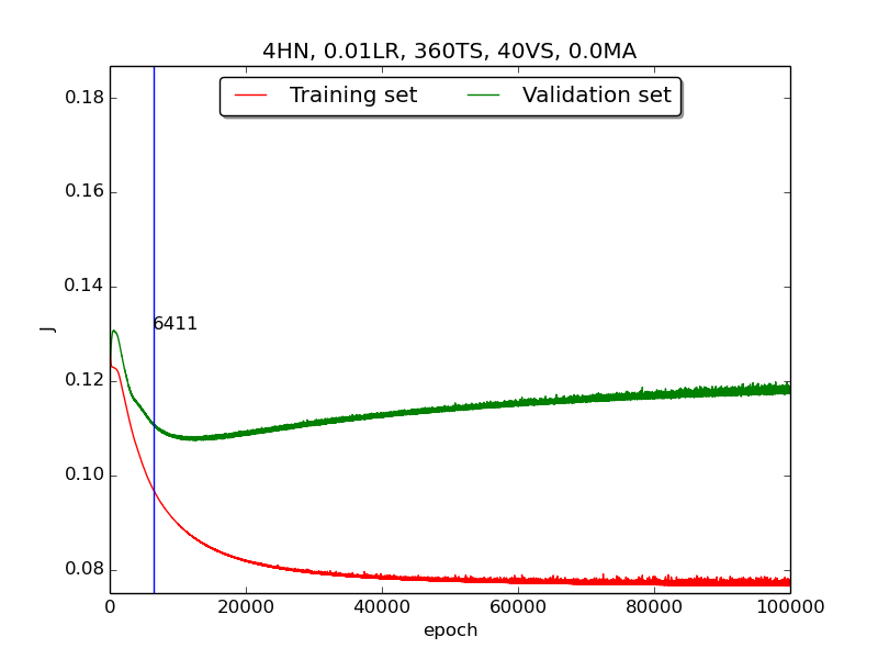 ↑ Results of running 100,000 epochs on a NN of 4 neurons in the hidden layer, 0.01 learning rate, 360 data points in training set, 40 data points in validation set and no momentum term
[4] For the
thirdpart, the four figures testified that the higher momentum is, the larger the amplitude of oscillation becomes.[5] However, in the
thirdpart, some unexpected results had shown. As far as I know, the higher momentum should have led to the increase of speed of convergence. Nevertheless, according to the figures inthrid, the least epoch satisfying early stopping criterion is when momentum = 0.4 instead of 0.8. I think the reason was the different (resulting from randomness) choice of initial biases.[6] As for normalization, I transformed all the points classified as
2to0due to the output of activtion function (between 0~1, inclusive).Ref / Note
[1] Code ref: A Step by Step Backpropagation Example – Matt Mazur
[2] Understanding Neural Network Batch Training: A Tutorial – Visual Studio Magazine
[3] Occam’s razor on Wikipedia
Source → cyhuang1230/NCTU_CI
Please look for
HW1.py.